Identifying a geochemical anomaly is the fundamental goal of mineral exploration, a complex, multidisciplinary science heavily reliant on detecting the “unseen.” At the heart of exploration campaigns is geochemistry. This process typically begins with stream sediment sampling on a regional scale and, as potential areas are narrowed down, transitions to denser, grid-based soil sampling. The ultimate objective of both methods is to pinpoint these anomalies—areas where the concentration of economically valuable elements is unusually high.
However, defining what constitutes an anomaly is not as simple as applying a universal mathematical rule. The Earth’s crust is highly heterogeneous. Therefore, assigning a single “global” threshold value to an entire study area often leads to false positives (wasted drilling budgets) and false negatives (missed massive ore deposits). This article examines the nature of anomalies in stream sediment and soil geochemistry and details why using a geological base map to dynamically adjust background values is an absolute necessity.
1. Decoding the Geochemical Anomaly and Dispersion Halos
A geochemical anomaly is a statistical deviation from the normal chemical background of a specific geological environment. To understand an anomaly, one must first understand the background. The background is the normal, natural concentration range of an element found in earth materials in an unmineralized area.
Stream sediment and soil geochemistry fall under the category of secondary anomalies. When a primary ore body underground weathers, elements mobilize toward the surface via groundwater, chemical dissolution, and physical erosion.
- In Soil: A “dispersion halo” carrying the signature of the ore forms in the soil directly above or adjacent to the deposit.
- In Stream Sediments: Materials washed from these soils are transported into streams, creating “drainage trains.”
2. The Two Workhorses of Exploration: Stream Sediments and Soil Sampling
A successful exploration program progresses from macro to micro. Understanding how these two environments reflect anomalies is essential for establishing accurate statistics:
A. Stream Sediment (Regional Screening)
Stream sediment sampling acts as a natural funnel. A single sample taken from an active stream bed is a physical and chemical composite of the rocks, soils, and vegetation of the entire catchment basin upstream. It is excellent for rapidly screening vast areas (e.g., 5,000 km²) and identifying “basins of interest.”
B. Soil (Target Definition)
Once a stream sediment anomaly highlights a potential basin, geologists mobilize to that area to collect soil samples on a systematic grid (e.g., at 100m x 50m intervals). Soil sampling is not a composite; it directly reflects the chemical signature of the underlying bedrock or the regolith (weathered zone). Its purpose is to pinpoint exactly where to position the drill rig.
How is the Threshold Determined?
In both methods, a threshold is established to separate the anomaly from the normal background. Traditionally, this is done via:
- Classical Statistics: Mean plus two standard deviations (μ + 2σ).
- Exploratory Data Analysis (EDA): Median Absolute Deviation (MAD) or Boxplots.
- Fractal Geometry (C-A Models): Plotting break points in the dataset.
However, if all these methods assume the data originates from a single rock type (a homogeneous population), they will lead the exploration program to disaster.
3. The Flaw of the “Global” Background Value

Table 1–Explanatory Note: The values presented in this table represent the natural, unmineralized background concentrations (baseline values) of trace elements commonly found in ordinary rock types. These numbers indicate the typical elemental abundance inherent to the rock’s original geological formation process, not the result of ore mineralization or hydrothermal alteration.
In the context of geochemical exploration, this data fundamentally demonstrates why a rock’s lithology must be considered when defining an “anomaly.” For instance, 200 ppm of Nickel would be a massive, drill-worthy anomaly in a granite terrain (where the natural background is only 4.5 ppm). However, the exact same 200 ppm value in an ultramafic terrain is actually depleted, as ordinary peridotite naturally contains around 2000 ppm Ni without any ore being present. This proves why anomaly thresholds must always be dynamically adjusted using a geological base map rather than relying on a single global value.
Applying a single threshold value (global threshold) across an entire project area is a geological error in both soil and stream sediment surveys. This is because different lithologies (rock types) have radically different natural background values.
Stream Sediment Example: Imagine surveying a 5,000 km² area. The software processes all nickel (Ni) data and sets the threshold at 80 ppm.
- An ultramafic rock (e.g., peridotite) in the region naturally contains 1500 ppm nickel. Every stream draining this rock will shine as an anomaly, leading you to “false positive” targets.
- Conversely, a felsic tuff in the region might host a genuine gold-nickel vein yielding 75 ppm Ni. Because the threshold is 80 ppm, this massive deposit will be overlooked (a false negative).
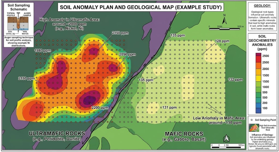
Soil Example: In a gold exploration project, you establish a soil grid over a 10 km² area. Half of the area consists of basalt (mafic), and the other half is rhyolite (felsic). You calculate a single threshold value for copper (Cu), say 60 ppm. Basalt has a natural soil background of 70-90 ppm Cu. Rhyolite, however, has a background of only 10-15 ppm Cu. When you plot the map, all the soils over the basalt will light up red (anomalous). But if there is an excellent 50 ppm ore leakage within the rhyolite, the statistics will deem it normal and hide it.
4. Dynamically Adjusting Anomaly Backgrounds using Geological Maps (GIS)

Picture 1: As you can see, while a nickel value of 2000 ppm for the ultramafic rocks on the left does not constitute an anomaly, a value of 130 ppm nickel for the mafic rocks on the right does not represent an anomaly either.
To strip mineral deposits from statistical noise, geochemical data must be reprocessed by overlaying it onto a geological base map. The background value is not a mathematical absolute; it is a geology-dependent variable. Using Geographic Information Systems (GIS), this is achieved as follows:
A. Lithological Subsetting (Pinpoint Accuracy for Soil Analyses)
In soil sampling, the exact rock unit under each sample point is known on the map (Point-in-Polygon analysis). Using the geological map, soil samples are subsetted based on their underlying bedrock. Separate thresholds are calculated for soils over basalt and soils over rhyolite. Thus, an 80 ppm value over basalt is deemed “ordinary,” while a 40 ppm value over rhyolite is flagged as a “definitive drill target.”
B. Catchment Basin Analysis and Weighting (for Stream Sediments)
Because stream sediments represent an entire basin rather than a single rock, this is more complex. Catchment polygons generated in GIS are intersected with the geological map. For instance, if a basin is 70% granite and 30% shale, the software ratios the known regional backgrounds of these two rocks to generate a mathematically weighted, custom threshold strictly for that specific stream sample. This flawlessly filters out geological noise.
C. Regolith and Transported Cover Filtering (Vital for Soil Exploration)
Geological maps (or more specifically, regolith maps) tell us whether a soil was formed “in situ (residual)” or if it was “transported” by alluvial, colluvial, or glacial deposits.
- In a residual soil (weathered directly from the rock below), 100 ppb Gold (Au) is a massive anomaly, indicating you are right on top of the ore.
- However, in a transported (alluvial) soil, 100 ppb Gold might indicate the source is kilometers away. Geological maps allow us to classify which soil anomalies are “in situ” and which are “transported,” fundamentally changing the interpretation of the threshold values.
D. Scavenging and Hydromorphic Environments
In both soils (especially in B-horizons and laterites) and stream beds, Iron (Fe) and Manganese (Mn) oxides act as “chemical sponges.” They attract dissolved metals in water. Geologists use geological and topographical maps to identify swamp-like environments, fault lines, and hydrological accumulation zones. By applying regression analyses to Fe and Mn values, “false” anomalies caused purely by Fe/Mn scavenging are cleaned out, leaving only the “pure” anomalies originating from the actual bedrock ore.
Conclusion
Whether screening massive basins on a regional scale with stream sediments or meticulously detailing a potential site with a soil grid, treating geochemical data as numbers independent of their geological context is the biggest trap in exploration projects.
An anomaly is strictly relative to the geological environment in which it resides. Utilizing geological base maps when calculating background and threshold values is not merely an analytical luxury; it is a necessity of modern geochemistry. By filtering data according to bedrock type (lithology), catchment basin ratios, and regolith (soil) structures, we can eliminate the statistical noise created by nature. This geology-centric approach prevents millions of dollars in misdirected drilling while serving as the key to discovering hidden, massive ore deposits that standard software would otherwise miss.